Most trading models fail before the model matters. The training set leaks the future, the labels overlap, and the score looks significant because nobody adjusted the t-statistic for that overlap. A gradient-boosted tree on a leaky dataset loses money as reliably as a linear model on the same dataset.
Hyperliquid is a good place to do this properly, because its fills contain more than price and size. Every fill says which account traded, whether it was the taker, whether it opened or closed a position, the position size before the fill, and whether a liquidation caused it. Centralized exchanges publish the aggressor side of a trade at most. They do not publish the account, the open or close direction, or the position. This guide builds a feature set from those fills, trains models that learn one bar at a time, and scores the forecasts in a way that tells signal from noise.
The data comes from three Dwellir sources that produce the same bars: the Hyperliquid gRPC API for the last few days and live data, indexed fills from the Hyperliquid Index for older history, and OHLCV candles for long price-only tests. The code is in the hyperliquid-grpc-ml example. We ran the gRPC snippets against Hyperliquid mainnet on 25 October 2026 and the Index snippets on 28 October 2026.
What You Build
| Step | Technique | File |
|---|---|---|
| Training set | 1-minute bars from gRPC fills, indexed fills, or candles | collect_bars.py, hl_index.py |
| Features | Rolling z-scores, flow imbalance, opening flow, liquidation pressure, range volatility | research.py |
| Labels | Forward returns that reach the model only after they exist | mlkit.ForwardLabels |
| Model | Recursive least squares with forgetting and ridge | mlkit.RLS |
| Scoring | Information coefficient, hit rate, Newey-West t | mlkit.score |
| Pairs | Kalman filter for a drifting hedge ratio | mlkit.KalmanBeta |
| Factors | PCA across coins, walk-forward PCA regression | mlkit.pca, mlkit.walk_forward_pcr |
| Live | The same model, warmed on history, learning on the live stream | live.py |
The models are short numpy classes rather than scikit-learn calls, so you can read each one in a few lines and run the same object in a backtest and on a live stream.
Why Fills over gRPC
Dwellir's gRPC gateway has two services. MarketStreaming serves typed live streams such as StreamBbo, StreamTrades, and StreamAllFills. HyperliquidL1Gateway serves the node's raw feeds, including StreamFills, which is the one this guide uses.
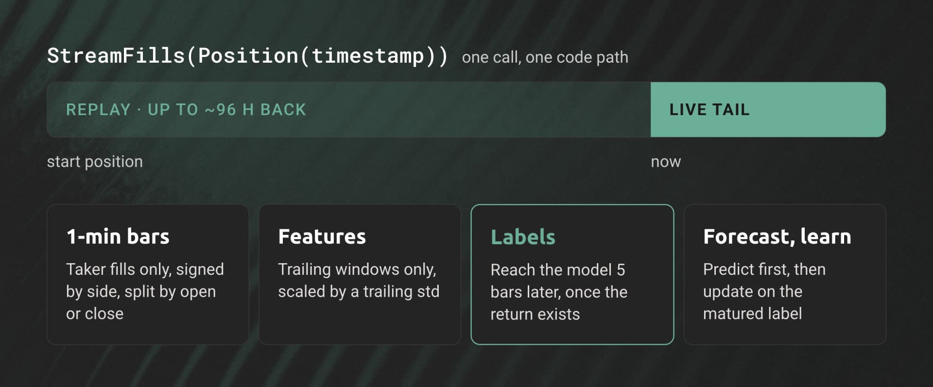
StreamFills takes a start position (a block number or a timestamp), replays every fill from that point, and then keeps streaming live on the same call. One loop builds the training set and then runs the model live, with no second data source and no join between a historical file and a live socket.
| Field in each fill | What it gives a model |
|---|---|
crossed | Whether this side was the taker, so you know who was aggressive |
side, px, sz | Signed taker flow |
dir | Open Long, Close Short, and so on: new risk versus risk leaving |
startPosition | The account's position before the fill |
liquidation | Set on fills caused by a liquidation, with the liquidated account and mark price |
closedPnl, fee | Realized PnL and fees per account |
user | The account, for wallet-level features |
The feed also takes a server-side filter, so you receive only the coins you ask for. The gRPC reference lists the other raw feeds: blocks, order statuses, raw book diffs, TWAP statuses, and misc events.
Three Sources for the Same Bars
The gRPC replay reaches back only a few days. For longer tests, the Hyperliquid Index serves the same fills and pre-built candles over HTTPS, back to 27 July 2025, with the same API key. collect_bars.py takes a --source flag, and research.py reads the result of any of the three.
gRPC StreamFills | Index allFillsByTime | Index candles | |
|---|---|---|---|
| History | About 96 hours back, then live | Back to 27 July 2025 | Back to 27 July 2025 |
| Bar columns | All: OHLC, taker buy and sell, opening flow, liquidations, trades | All, with liquidations joined from liquidationFillsByTime | OHLC, notional, trade count |
| Cost | 1 credit per block with a matching fill | 1 credit per fill returned | 1 credit per candle |
| Measured speed | 72 hours of 8 coins in 12 minutes | About 1,000 fills per second | 90 days of 8 coins in 5 minutes |
| Use it for | Recent history and the live model | Flow features on older dates | Long price and volume tests |
We checked that the three agree. For BTC and ETH from 12:00 to 13:00 UTC on 23 October 2026, bars built from indexed fills matched the gRPC bars exactly on every column: OHLC, notional, taker buy notional, opening flow, and trade count. Candles matched on OHLC, notional, and trade count; the candle trade count is the number of taker fills. For an hour with $34.3 million of BTC long liquidations (15:00 UTC on 24 October), the liquidation columns from the Index also matched the gRPC bars.
Prerequisites
You need Python 3.10 or later and a Dwellir API key. The gRPC path needs the Hyperliquid gRPC add-on and the generated stubs below. The Index paths need only the key.
git clone https://github.com/dwellir-public/dwellir-examples
cd dwellir-examples/examples/hyperliquid-grpc-ml
python3 -m venv .venv && source .venv/bin/activate
pip install -r requirements.txt

curl -fsSLo v3.proto https://www.dwellir.com/docs/hyperliquid/grpc/v3.proto
python -m grpc_tools.protoc -I. --python_out=. --grpc_python_out=. v3.proto

export DWELLIR_API_KEY=your-api-key
Step 1: Build the Training Set from Replayed Fills
The stream reader runs in its own thread and puts raw records on a queue. Parsing happens on the main thread. Our first version parsed inside the receive loop, and the 24-hour replay stalled after about 200,000 fills with the client idle. With a separate reader thread, the same replay finished in 4 minutes. Drain first, parse second.
def _read_fills(coins, start_ms, records):
    channel, metadata = connect()
    gateway = rpc.HyperliquidL1GatewayStub(channel)
    flt = pb.Filter(fields=[pb.FieldFilter(field="coins", values=coins)])
    position = pb.Position(timestamp=start_ms)
    last_block, backoff = None, 1
    while True:
        try:
            request = pb.StreamRequest(position=position, filter=flt)
            for record in gateway.StreamFills(request, metadata=metadata):
                if last_block is not None and record.block_number <= last_block:
                    continue  # positions are inclusive; skip the block we already have
                last_block, backoff = record.block_number, 1
                records.put((record.block_number, record.timestamp, record.data))
        except grpc.RpcError as err:
            if err.code() not in RETRY_CODES:
                records.put(err)  # the parsing side re-raises it
                return
            if last_block is not None:
                position = pb.Position(block_number=last_block)  # resume where we stopped
            time.sleep(backoff)
            backoff = min(backoff * 2, 30)
Each record is one block's fills as JSON. Every match produces two fills, one per side, so the bar builder counts only the taker side (crossed: true). That counts each trade once and signs it by the aggressor:
if not fill.get("crossed"):
    return
ntl = float(fill["px"]) * float(fill["sz"])
buy = fill["side"] == "B"
bar["buy_ntl" if buy else "sell_ntl"] += ntl
if fill["dir"].startswith("Open"):
    bar["open_buy_ntl" if buy else "open_sell_ntl"] += ntl
if fill.get("liquidation"):
    # A forced sell closes a long, a forced buy closes a short.
    bar["liq_short_ntl" if buy else "liq_long_ntl"] += ntl
Replay 72 hours of 8 coins into 1-minute bars:
python collect_bars.py --hours 72 --coins BTC,ETH,SOL,HYPE,XRP,DOGE,SUI,BNB --out bars.parquet 1.9% 100,000 fills 652 bars 14s
4.6% 200,000 fills 1,570 bars 33s
...
97.4% 4,000,000 fills 33,073 bars 699s
4,051,862 fills -> 33,967 bars for 8 coins -> bars.parquetThe 72-hour replay took 12 minutes and 24 hours took 4. The filtered stream sends one message per block that has a matching fill, and each message costs 1 API credit. For these 8 coins we measured 10,216 messages for one hour, so 72 hours is roughly 700,000 credits.
How far back you can go. The raw feeds keep a rolling window. On 25 October 2026, StreamFills replayed about 96 hours; a start time before that returned NOT_FOUND: Data for provided timestamp is pruned. The window varies by feed and endpoint. For older dates, use the Index.
Older Fills from the Index
allFillsByTime returns indexed fills for one coin inside a window of at most 1 hour, up to 2,000 per page. The response is a bare array, so you build the next cursor from the last fill's time and txIndex:
def _by_time(kind, start_ms, end_ms, coin=None):
    for hour in range(start_ms, end_ms, HOUR_MS):
        body = {"type": kind, "startTime": hour, "endTime": min(hour + HOUR_MS, end_ms), "limit": 2000}
        if coin:
            body["coin"] = coin
        while True:
            fills = _request(_url("/info"), body)
            yield from fills
            if len(fills) < 2000:
                break                                   # a short page ends the hour
            body.pop("startTime", None)
            body["cursor"] = f"{fills[-1]['time']}_{fills[-1]['txIndex']}"
Indexed fills have the same fields as StreamFills, including both sides of each match and the crossed flag, but no liquidation field. index_fills takes that from liquidationFillsByTime and joins it on the trade id, so the same BarBuilder reads both sources:
liq = {f["tid"]: f["liquidation"] for f in _by_time("liquidationFillsByTime", hour, stop, coin)}
for fill in _by_time("allFillsByTime", hour, stop, coin):
    if fill.get("tid") in liq:
        fill["liquidation"] = liq[fill["tid"]]
yield fillpython collect_bars.py --source index --coins BTC,ETH --start 2026-09-01 --end 2026-09-08 --out bars_sep.parquetEach fill returned costs 1 credit, and every match returns two fills. BTC alone returned 23,696 fills in a quiet hour and 94,772 in an hour with heavy liquidations, so one day of BTC is in the hundreds of thousands of credits. For the last 96 hours, the gRPC replay is much cheaper, because it bills per block rather than per fill. Use the Index for dates the replay cannot reach.
Candles for Long Price-Only History
When a model needs price and volume but not taker flow, candles cost far less. The candle range endpoint returns up to 5,000 1s, 1m, or 5m candles per page:
python collect_bars.py --source candles --start 2026-07-29 --end 2026-10-27 --out candles90.parquetBTC 129,574 candles
ETH 129,571 candles
...
BNB 125,036 candles
1,025,218 candles -> 1,025,218 bars for 8 coins -> candles90.parquetThat is 90 days of 8 coins in 5 minutes, for about 1 million credits. Candles are sparse: a minute with no trades has no candle, and to_grid fills it with the last close. For the whole archive of one market in one file, generate a full-history export (CSV or Parquet) from the dashboard and read it with hl_index.load_export(path).
A candle does not record which side was the aggressor, so the flow columns are missing. research.py detects that and switches to price inputs: the last 1- and 5-minute returns, ret_z_30, and a notional z-score.
The Hyperliquid historical data archive has the raw node_fills_by_block files if you would rather process files yourself. Hyperliquid historical data for backtesting compares 20 sources of history.
Step 2: Rolling Statistics
Features are rolling statistics over the bars. They follow pandas conventions, so a number you check in a notebook matches the number the model sees. Variance divides by n - 1.
def zscore(s, n):
    return (s - s.rolling(n).mean()) / s.rolling(n).std()

def imbalance(a, b, n):
    """(a - b) / (a + b) over the last n bars. 0 when nothing traded."""
    num = a.rolling(n).sum() - b.rolling(n).sum()
    den = a.rolling(n).sum() + b.rolling(n).sum()
    return (num / den).where(den > 0, 0.0)

def parkinson_vol(high, low, n):
    return np.sqrt((np.log(high / low) ** 2).rolling(n).mean() / (4 * np.log(2)))

f["flow_5"]       = imbalance(b.buy_ntl, b.sell_ntl, 5)            # taker buy vs sell, 5 min
f["open_flow_15"] = imbalance(b.open_buy_ntl, b.open_sell_ntl, 15) # new longs vs new shorts
f["liq_15"]       = (b.liq_short_ntl - b.liq_long_ntl).rolling(15).sum() / b.notional.rolling(15).sum()
f["ret_z_30"]     = zscore(np.log(b.close), 30)                    # stretch from the 30-min mean
f["vol_30"]       = parkinson_vol(b.high, b.low, 30)
open_flow_15 needs account-level fill data, which Hyperliquid publishes and centralized exchanges do not. Taker buying that opens new longs is a different event from taker buying that closes shorts, and the dir field separates them. liq_15 measures forced flow as a share of all flow.
Step 3: The Lookahead Trap
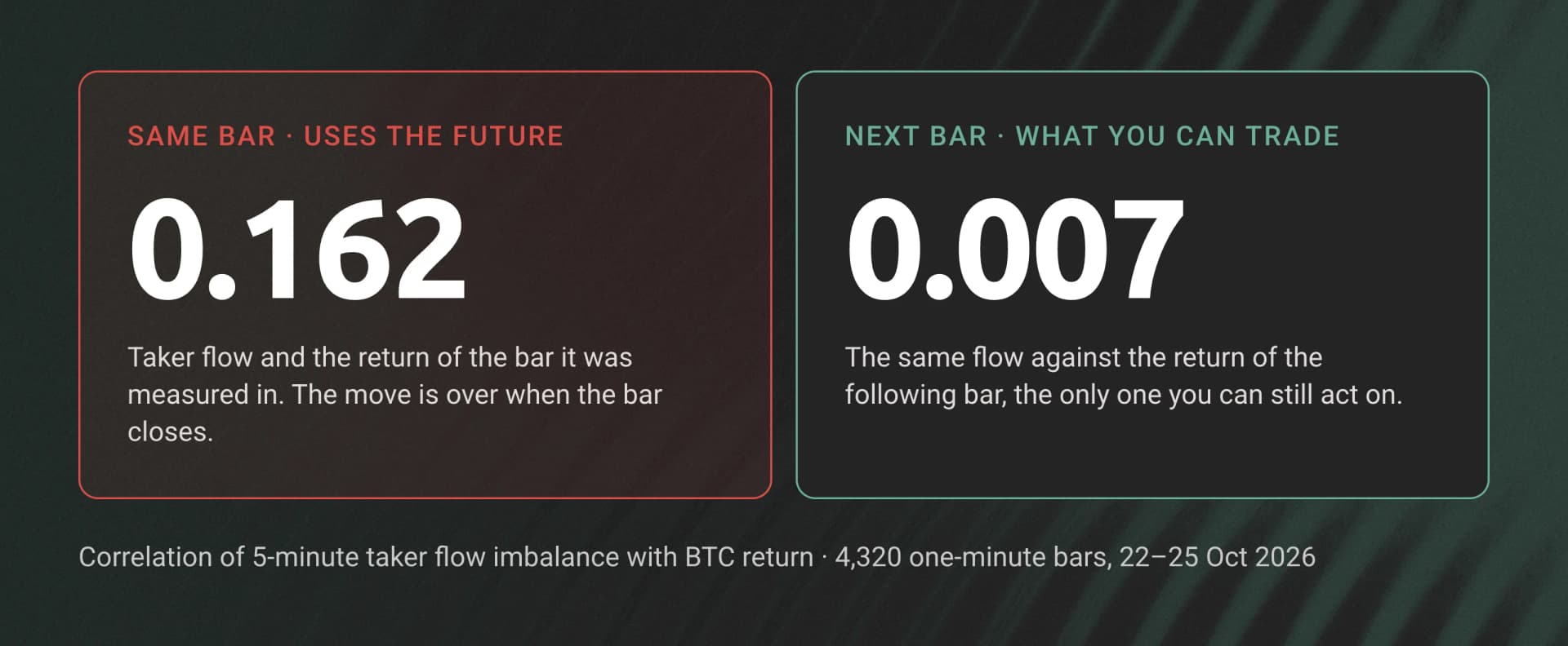
The fastest way to fool yourself is to correlate a feature with the return of the same bar. Taker buying and price rise happen together, so the correlation is high and useless: by the time the bar closes, the move is over.
corr(flow_5, return of the same bar) = +0.162   <- uses the future
corr(flow_5, return of the next bar) = +0.007   <- what you can trade
Over 4,320 BTC bars, 5-minute taker flow imbalance correlates at 0.162 with the return of the bar it was measured in and 0.007 with the next bar. A model trained on the first number looks brilliant in a backtest and has nothing to trade. Candles have the same trap: over 90 days, ret_z_30 correlates at 0.319 with the same bar's return and 0.000 with the next. Every label below starts after the bar whose features produced it.
Step 4: Labels a Model Cannot See Early
A model needs the return that followed each reading, and that return does not exist until h bars later. ForwardLabels stores each bar's inputs and returns them with the label only once the label exists:
class ForwardLabels:
    def __init__(self, h):
        self.h = h
        self.queue = deque()

    def update(self, x, price):
        self.queue.append((x, price))
        if len(self.queue) <= self.h:
            return None
        x_then, price_then = self.queue.popleft()
        return x_then, float(np.log(price / price_then))
Train only on what update returns and the model cannot learn from the future, in a backtest or live. The same rule applies to any preprocessing: scale inputs by a trailing standard deviation, not by the standard deviation of the whole dataset.
Step 5: Regression That Learns Bar by Bar
Recursive least squares (RLS) updates a linear regression one observation at a time. A forgetting factor down-weights old bars so the coefficients follow a market that changes, and ridge keeps them steady when inputs move together.
class RLS:
    def __init__(self, n_inputs, forget=0.995, ridge=1.0):
        self.forget = forget
        self.w = np.zeros(n_inputs + 1)
        self.P = np.diag([1e6] + [1.0 / ridge] * n_inputs)  # ridge on slopes, not the intercept

    def predict(self, x):
        return float(self.w @ np.r_[1.0, x])

    def update(self, y, x):
        z = np.r_[1.0, x]
        fitted = float(self.w @ z)
        Pz = self.P @ z
        k = Pz / (self.forget + z @ Pz)
        self.w = self.w + k * (y - fitted)
        self.P = (self.P - np.outer(k, Pz)) / self.forget
        self.P = (self.P + self.P.T) / 2                     # stop rounding drift
        return fitted, y - fitted
The training loop forecasts first, then learns from the label that has just become available:
labels, model = ForwardLabels(5), RLS(4, forget=0.998, ridge=10)
for t, (x, px) in enumerate(zip(X.to_numpy(), b.close.to_numpy())):
    forecast[t] = model.predict(x)          # made before this bar's label exists
    done = labels.update(x, px)
    if done is not None:
        model.update(done[1], done[0])      # learn from the bar 5 minutes ago
forget=0.998 gives a half-life of about 350 bars, close to 6 hours of 1-minute data. Give the inputs similar scales before you apply ridge; research.py divides each by its trailing 4-hour standard deviation.
The symmetrize line matters on long runs. On 72 hours of bars the model worked without it. On 90 days of candles, rounding errors in P grew until one forecast reached -14,416 against a typical size of 0.003, and that one bar pushed the t-statistics as high as 200. Re-symmetrizing P after each update kept it stable, and the 72-hour results did not change.
Step 6: Scoring a Forecast
Three numbers grade a forecast against the h-bar return that followed it:
- IC (information coefficient): the correlation between forecast and return.
- Hit rate: the share of bars where forecast and return have the same sign, skipping bars where the price did not move.
- t: the t-statistic of the return's slope on the forecast.
The t-statistic needs care. A 5-bar return sampled every bar shares 4 bars with the next one, so consecutive errors are correlated and an ordinary t-statistic overstates confidence by roughly the square root of 5. Newey-West standard errors with h - 1 lags correct for that overlap:
def newey_west_t(f, r, lags):
    X = np.column_stack([np.ones_like(f), f])
    XtX_inv = np.linalg.inv(X.T @ X)
    beta = XtX_inv @ X.T @ r
    Xu = X * (r - X @ beta)[:, None]
    S = Xu.T @ Xu
    for lag in range(1, lags + 1):
        G = Xu[lag:].T @ Xu[:-lag]
        S += (1 - lag / (lags + 1)) * (G + G.T)
    V = XtX_inv @ S @ XtX_inv
    return beta[1] / np.sqrt(V[1, 1])
The online RLS model on BTC, scored at 1, 5, and 15 minutes:
        ic     hit       t     n
h
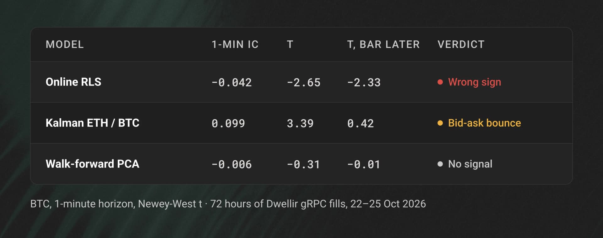
1  -0.0425  0.4859 -2.6540  4225
5  -0.0671  0.4869 -2.4449  4221
15 -0.0690  0.4961 -1.6811  4211
The model is wrong more often than it is right, and at 1 and 5 minutes the t-statistic says that is not chance. Score each input on its own, day by day, and you see why. open_flow_15 correlated with the next 5-minute return at +0.156 on 22 October and at -0.093 on 23 October. ret_z_30 went from -0.124 to +0.072 over the four days. A model that learns from the past picks up the sign that just stopped working. Slower forgetting does not fix it: with forget=1.0, which weighs every past bar equally, the 1-minute IC is still -0.036.
You could flip the sign and report a positive IC, but that is a decision made after seeing the test data. Treat it as a hypothesis and test it on days the model has not seen.
One more check catches a common false positive. Score the forecast as if you could only trade on the bar after it (score(forecast, close, delay=1)). The last trade price bounces between the bid and the ask, and that bounce alone creates short-term mean reversion that nobody can capture. The RLS result survives the delay (1-minute IC -0.039, t -2.33). The Kalman signal in the next step does not.
Step 7: A Kalman Filter for a Drifting Hedge Ratio
A pairs trade needs a hedge ratio, and a ratio fitted once goes stale. A Kalman filter treats the intercept and slope of log(ETH) = alpha + beta * log(BTC) as random walks and updates both every bar. Its surprise on each bar is the spread, and dividing by the filter's own uncertainty gives a z-score:
class KalmanBeta:
    def __init__(self, delta=1e-8, obs_var=1e-7, init_var=1e-2):
        self.theta = np.zeros(2)                    # alpha, beta
        self.P = init_var * np.eye(2)
        self.Q = delta / (1 - delta) * np.eye(2)    # how fast alpha and beta may drift
        self.R = obs_var                            # noise around the line

    def update(self, y, x):
        z = np.array([1.0, x])
        self.P = self.P + self.Q
        spread = y - z @ self.theta                 # surprise, from before this bar
        S = z @ self.P @ z + self.R
        K = self.P @ z / S
        self.theta = self.theta + K * spread
        self.P = self.P - np.outer(K, z) @ self.P
        return {"beta": self.theta[1], "spread": spread, "z": spread / np.sqrt(S)}

kf = KalmanBeta(delta=1e-8, obs_var=1e-7, init_var=1e-2)
y, x = np.log(eth.close / eth.close.iloc[0]), np.log(btc.close / btc.close.iloc[0])
k = pd.DataFrame([kf.update(yi, xi) for yi, xi in zip(y, x)], index=btc.index)
Divide each price by its first value before taking logs. Raw log prices sit near 11.3 for BTC, which makes the intercept and slope almost impossible to tell apart. Tune delta and obs_var until the z-score has a standard deviation near 1; we picked these values on the most recent 24 hours of the data by checking that calibration, not by maximizing the score.
beta: start 0.990, end 1.378, range 0.980 to 1.384
z std 0.98, |z| > 2 on 4.0% of bars

forecast = -z, scored on the hedged pair return that followed:
        ic     hit       t     n
1   0.0991  0.5461  3.3886  4199
5   0.0702  0.5246  1.9623  4195
15  0.0597  0.5390  1.0648  4185

the same, trading one bar after the signal:
1   0.0130  0.5050  0.4169  4198
5   0.0164  0.5123  0.4297  4194
15  0.0240  0.5250  0.3907  4184
ETH's beta to BTC moved from 0.99 to 1.38 over three days, which a fixed hedge ratio would have missed. The z-score is calibrated: 4.0% of bars beyond 2, against 4.6% for a normal distribution.
The first score table looks like a tradeable pairs signal, with a 1-minute IC of 0.099 and a t-statistic of 3.39. Start the return one bar later and the IC falls to 0.013 with a t of 0.42. The edge was bid-ask bounce in the last trade price: a z-score computed from a trade at the ask predicts that the next trade is more likely at the bid. To test whether the spread mean-reverts, compute it from mid prices, which you can record from StreamBbo on the same API.
Step 8: Principal Components across Coins
PCA finds the directions in which a set of series move together. Run it on 1-minute returns of the 8 coins and the first component is the market factor:
share of variance: [0.745 0.061 0.049]
        PC1    PC2    PC3
BNB   0.310  0.853 -0.385
BTC   0.368 -0.098 -0.199
DOGE  0.345  0.124  0.563
ETH   0.376 -0.133 -0.129
HYPE  0.328 -0.462 -0.514
SOL   0.379 -0.112 -0.006
SUI   0.353 -0.011  0.423
XRP   0.362 -0.064  0.190
The first component explains 74.5% of the variance in 1-minute returns, with every coin loading between 0.31 and 0.38: when the market moves, everything moves. The second component is mostly BNB against HYPE, and the third sets DOGE and SUI against HYPE and BNB. For a single-coin model, removing the PC1 score from a coin's return leaves its idiosyncratic move, which is often a better target.
mlkit.pca standardizes the inputs, computes the components exactly from the covariance matrix, and flips each component so its largest loading is positive. Without that flip, a component can change sign between two fits, and any model trained on its scores suddenly reads the opposite signal.
Step 9: Walk-Forward PCA Regression
A model that keeps learning from PCA scores has a problem: every refit moves the components under it, and when two small components swap order, its coefficients apply to the wrong one. Principal component regression (PCR) avoids that by fitting the components and the regression on them together, then freezing both until the next refit.
Done walk-forward, each stretch is forecast by a fit that saw only the bars before it. The training window ends h bars before the refit, because the labels of the last h bars do not exist yet:
for t in range(window + h, len(A), refit):
    train = slice(t - h - window, t - h)          # labels that exist at time t
    p = pca(A[train], k)
    scores = ((A[train] - p["mu"]) / p["sd"]) @ p["loadings"]
    coef = ols(scores, Y[train])
    ahead = slice(t, t + refit)                   # frozen until the next refit
    out[ahead] = coef[0] + (((A[ahead] - p["mu"]) / p["sd"]) @ p["loadings"]) @ coef[1:]
The inputs are a ladder of taker-flow imbalances over 1 to 34 minutes and return z-scores over 5 to 60 minutes, 12 series that overlap heavily. PCA compresses them to 3 components:
59 refits; PC1 share at first/last refit: 0.52 / 0.53
        ic     hit       t     n
h
1  -0.0061  0.5062 -0.3106  3535
5   0.0100  0.5134  0.3092  3531
15  0.0102  0.5091  0.2357  3521
The walk-forward forecast finds nothing. Over 59 refits and 3,535 out-of-sample bars, its IC is near 0 and no t-statistic reaches 0.32. Price and flow features of BTC alone, compressed or not, do not forecast BTC at these horizons over these three days. Before you add a gradient-boosted model, add information the market price does not already contain, such as book depth from StreamL2Book, wallet-level flows from the user field, or liquidation levels.
All three models side by side, at the 1-minute horizon:
Step 10: Repeat the Tests on 90 Days of Candles
Three days is a short test. The same research.py run on 90 days of 1-minute candles (29 July to 27 October 2026, 129,600 BTC bars) repeats each test on a window 30 times longer:
python research.py candles90.parquet --coin BTC --pair ETH| Model | 1-min IC | t | t, one bar later | Result over 90 days |
|---|---|---|---|---|
| Online RLS, price inputs | -0.0074 | -1.18 | -1.97 | Weak, borderline only when delayed |
| Kalman ETH / BTC | 0.0623 | 3.19 | 0.86 | Bid-ask bounce again |
| Walk-forward PCA, 2,146 refits | -0.0109 | -0.94 | -0.70 | No signal |
The Kalman pattern repeats: a t of 3.19 at the last trade price, falling to 0.86 one bar later. The same drop over 129,000 bars fits bid-ask bounce, not a spread that reverts. ETH's beta to BTC moved from 0.92 to 1.32 over the 90 days. The z-score standard deviation was 1.35, against 0.98 on the 72 hours, because the filter was tuned on the short window; tune it again on the longer one.
PC1 explains 67.9% of the variance in 1-minute returns over 90 days, against 74.5% over the 3 days. The second component over 90 days is almost entirely HYPE, with a loading of 0.91. The online RLS here uses price inputs only, so it is a different model from the flow model in Step 6. To retest the flow model on older dates, collect bars with --source index instead.
Step 11: Run It Live
live.py replays the last 6 hours to warm the model, crosses into live data on the same StreamFills call, and prints a forecast on every closed bar next to the return that followed the forecast made 5 minutes earlier:
python live.py --coin BTC --warmup-hours 6replay 2026-10-25 16:12 60 bars learned
replay 2026-10-25 17:12 120 bars learned
replay 2026-10-25 18:12 180 bars learned
replay 2026-10-25 19:12 240 bars learned
19:45 BTC 80,574.0 next 5m forecast -0.97 bp | 5m ago said -2.04 bp, got +1.61 bp
19:46 BTC 80,569.0 next 5m forecast -0.87 bp | 5m ago said -1.96 bp, got +0.99 bp
19:47 BTC 80,558.0 next 5m forecast -0.54 bp | 5m ago said -1.15 bp, got -0.37 bp
19:48 BTC 80,558.0 next 5m forecast -0.60 bp | 5m ago said -1.43 bp, got -1.61 bpThe forecasts are around 1 basis point. Hyperliquid's base perp taker fee is 0.045%, or 4.5 basis points, so even a correct forecast of this size loses money as a taker trade. That matches the scores above. Swap in better features and the same loop trains on history and runs live.
The model keeps learning live with the same ForwardLabels and RLS objects it used on history. Nothing changes at the boundary between replay and live data, because one code path handles both.
Production Notes
- Drain the stream before you parse. Parsing inside the receive loop stalled our replay; a separate reader thread fixed it. Read on one thread, parse on another.
- Resume from the last block. On
UNAVAILABLE,DEADLINE_EXCEEDED,DATA_LOSS, orRESOURCE_EXHAUSTED, reconnect withPosition(block_number=last_block)and skip that block, since positions are inclusive. - Expect silence. The raw feeds send no heartbeats. A filtered stream on a quiet coin can be silent and healthy. Opt in to progress frames with
StreamRequest.progressif you need a liveness signal. - Count the cost. Each streamed gRPC message costs 1 API credit, and a filtered stream sends one message per block that has a matching fill. Index fills cost 1 credit per fill and candles 1 credit per candle. Use gRPC for the last 96 hours, indexed fills for older flow data, and candles when price is enough.
- Test for longer. One day of 1-minute bars is about 1,440 rows per coin. Use candles or indexed fills to test across months before you trust an IC.
- Keep online models numerically stable. An RLS that runs for 100,000 bars or more needs its covariance re-symmetrized, or one bad forecast can dominate the score.
Frequently Asked Questions
What data do I need to train an ML model on Hyperliquid?
For order-flow models, fills are the richest source: every fill has price, size, the taker flag, whether it opened or closed a position, and whether a liquidation caused it. Dwellir's gRPC StreamFills replays recent fills and then streams live, and the Hyperliquid Index serves the same fills back to July 2025. For price-only models, 1-minute candles are cheaper. For order book features, add StreamL2Book or StreamBbo.
How far back can I get Hyperliquid fills and candles?
The gRPC StreamFills replay reached about 96 hours back on 25 October 2026; an older start position returns NOT_FOUND. The Hyperliquid Index serves fills (allFillsByTime) and 1s, 1m, and 5m candles back to 27 July 2025. For raw node files, use the historical data archive.
Can I train a model on candles instead of fills?
Yes, for price and volume features. A candle has open, high, low, close, volume, notional, and trade count, but not the taker side, the open or close direction, or liquidations, so flow features need fills. In this guide's tests, candles and fills gave identical prices, notional, and trade counts for the same minutes.
Why are my backtest results better than my live results?
Usually lookahead or overlap. Check that no feature uses the current bar's return, that labels reach the model only after they exist, that scaling uses trailing statistics, and that t-statistics on overlapping labels use Newey-West or a similar correction.
What IC is good for a 1-minute crypto forecast?
Small numbers are normal at 1 minute. What matters is whether the IC keeps its sign on days the model has not seen, survives a one-bar delay, and implies moves larger than your trading costs. In this guide's live run, forecasts of about 1 basis point were well below the 4.5-basis-point taker fee. A high IC on one day is more likely noise, bid-ask bounce, or leakage.
Can I use scikit-learn or PyTorch instead?
Yes. The bars are a pandas DataFrame, so any library works. Keep ForwardLabels (or an equivalent purge and embargo) and the walk-forward split, because the leakage problems come from the data handling, not the model.
Start Building
Clone the hyperliquid-grpc-ml example and create a Dwellir account. The candle and indexed-fill paths run with the API key alone; enable the Hyperliquid gRPC add-on for the replay and the live model. For dedicated Hyperliquid nodes with unmetered gRPC, or archive data beyond the replay window, contact the Dwellir team.