Most candle data APIs on Hyperliquid bottom out at 1-minute intervals. That works fine until you try to backtest an execution algorithm and realize 60 seconds of price action got compressed into a single bar. The wick that would have triggered your stop? Invisible. The 3-second liquidity sweep that moved price 2% and snapped back? Averaged away.
For anything beyond casual charting, 1-minute candles hide more than they reveal.
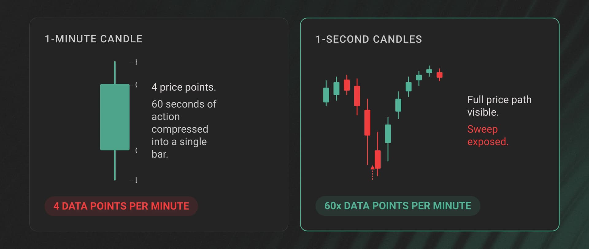
The gap between 1-minute and 1-second resolution isn't a minor upgrade. It's the difference between "price went from A to B" and "price went from A to C to D to B, sweeping liquidity at C along the way." If you're building trading infrastructure, execution analytics, or ML models on Hyperliquid, the granularity of your candle data determines the ceiling of what you can build.
Dwellir provides pre-aggregated OHLCV candlestick data for Hyperliquid at 1-second, 1-minute, and 5-minute intervals - covering perps, spot, and HIP-3 perpDex markets through a single unified schema. This article walks through 7 concrete things you can build with that data, with code examples showing how to pull it.
The Dwellir OHLCV API at a Glance
Before jumping into use cases, here's what the API provides.
Dwellir aggregates OHLCV candles directly from raw fills on Hyperliquid. The data covers all market types through a unified schema:
| Market Type | Symbol Format | Example |
|---|---|---|
| Perps | Ticker | BTC, ETH, SOL |
| Spot | @ + asset ID | @142 |
| HIP-3 perpDex | deployer:TICKER | hyna:ETH, xyz:AAPL |
Each candle includes the standard OHLCV fields plus trade count (n), quote notional volume (q), and a finalization flag (x).
Two access patterns cover both historical analysis and live streaming. The REST endpoint fetches a single candle by market, interval, and timestamp:
# Fetch a 1-minute BTC candle for a specific timestamp
curl "https://api-hyperliquid-index.n.dwellir.com/YOUR_API_KEY/v1/candles?market=BTC&interval=1m&time=2026-03-30T23:00:00Z"
The WebSocket endpoint streams live candle updates with partial (open) and finalized states:
{
  "type": "subscribe",
  "market": "BTC",
  "interval": "1s"
}
The WebSocket feed includes seq and cursor fields for gap detection. If you miss a message, you know exactly where to backfill from. Historical coverage begins in mid-2025.
Here are 7 things worth building with this data.
1. Algo Trading Backtester With Realistic Slippage
Standard backtesting on 1-minute candles assumes you can execute at any price between the open and close. That produces results that look great in a spreadsheet and fall apart in production. A 1-minute bar compresses dozens of microstructure events - liquidity sweeps, momentum bursts, mean reversions - into 4 price points.
With 1-second candles, your backtester can simulate fills against a much more granular price path. Because candles are built from executed trades, the high and low values reflect actual fill prices - not order book midpoints or theoretical marks. This matters for slippage modeling: if a sweep pushed price 1.5% below the 1-minute low before recovering, your backtester sees that and accounts for it.
You can pull a range of 1-second candles for backtesting by iterating over timestamps:
import requests
from datetime import datetime, timedelta

API_KEY = "YOUR_API_KEY"
BASE_URL = f"https://api-hyperliquid-index.n.dwellir.com/{API_KEY}/v1/candles"

def fetch_candles(market, interval, start, end):
    """
    Fetch candles one at a time across a time range.

    Note: This illustrates the schema and access pattern. In production,
    you'd use batch/range endpoints or parallel requests for efficient ingestion.
    """
    candles = []
    current = start
    delta = timedelta(seconds=1) if interval == "1s" else timedelta(minutes=1)

    while current < end:
        resp = requests.get(BASE_URL, params={
            "market": market,
            "interval": interval,
            "time": current.isoformat() + "Z"
        })
        data = resp.json()
        if data:  # Sparse - no response for empty intervals
            candles.append(data)
        current += delta
    return candles

# Fetch 1-second BTC candles for a 10-minute window
candles = fetch_candles(
    market="BTC",
    interval="1s",
    start=datetime(2026, 3, 30, 23, 0, 0),
    end=datetime(2026, 3, 30, 23, 10, 0)
)
One detail worth flagging: Dwellir returns sparse candles, meaning intervals with zero trades return no data rather than a zero-volume placeholder bar. Your backtester doesn't need to filter out synthetic bars - if a candle exists, real trades happened during that second.
This has implications for downstream pipelines: if your system expects a continuous time series (e.g., for ML feature alignment or joins), you'll need to handle gaps explicitly - either forward-filling the last known close or resampling to a regular grid before processing.
2. Real-Time Trading Dashboard
A trading dashboard needs two things: historical context on page load and live updates as new candles form. The typical approach requires one data source for history and another for live data, with a stitching layer to merge them. Dwellir's REST + WebSocket combination handles both through the same schema.
On page load, fetch the last N candles via REST to populate the chart, then open a WebSocket connection to stream updates. The WebSocket sends two types of messages per candle: partial updates while the candle is still open (x: false) and a final message when the interval closes (x: true). Your frontend can update the current bar in real time without waiting for it to close.
// Simplified example - production usage requires API key authentication
const ws = new WebSocket("wss://api-hyperliquid-index.n.dwellir.com");

ws.onopen = () => {
  ws.send(JSON.stringify({
    type: "subscribe",
    market: "BTC",
    interval: "1s"
  }));
};

ws.onmessage = (event) => {
  const candle = JSON.parse(event.data);

  if (candle.x) {
    // Candle finalized - append to chart history
    appendCandleToChart(candle);
  } else {
    // Candle still open - update the live bar
    updateCurrentBar(candle);
  }
};
The seq field on each WebSocket message increments sequentially. If your client detects a gap in sequence numbers - say it received seq: 1042 followed by seq: 1044 - you know a message was dropped. Use the cursor value from your last received message to backfill the gap via REST before resuming the stream.
3. Cross-Market Spread and Arbitrage Monitor
Hyperliquid runs three distinct market types: perpetual futures, spot markets, and HIP-3 perpDex markets. Spread opportunities exist between them - the BTC perp price versus spot, or between two HIP-3 deployers listing the same asset. Monitoring these spreads requires candle data from all market types in a format you can directly compare.
Dwellir serves all three market types through the same OHLCV schema. A BTC perp candle has the same fields as a @142 spot candle or an hyna:ETH HIP-3 candle. No normalization layer needed. You subscribe to multiple markets over a single WebSocket connection and calculate spreads on every tick.
import json
import websockets
import asyncio

async def monitor_spread():
    uri = "wss://api-hyperliquid-index.n.dwellir.com"
    async with websockets.connect(uri) as ws:
        # Subscribe to both perp and spot for the same asset
        for market in ["ETH", "@142"]:  # ETH perp and spot
            await ws.send(json.dumps({
                "type": "subscribe",
                "market": market,
                "interval": "1s"
            }))

        prices = {}
        async for msg in ws:
            candle = json.loads(msg)
            symbol = candle["s"]
            prices[symbol] = float(candle["c"])  # Latest close price

            if len(prices) == 2:
                spread = prices["ETH"] - prices["@142"]
                spread_bps = (spread / prices["@142"]) * 10_000
                print(f"ETH perp-spot spread: {spread_bps:.1f} bps")

asyncio.run(monitor_spread())
At 1-second resolution, you catch spread dislocations that collapse within seconds. While spread monitoring works at longer intervals too, 1-second data lets you observe the full lifecycle of short-lived dislocations rather than only seeing them if they persist for an entire minute.
4. ML Price Prediction and Signal Generation
Machine learning models for price prediction are only as good as their training data. Two properties of Dwellir's candle data matter for ML pipelines: sparse semantics and enriched fields.
Most data providers pad empty intervals with zero-volume candles - synthetic bars where open equals close and volume is zero. These aren't "no movement" signals. They're "no data" signals. A model trained on padded data learns that zero-volume flat candles are a real market state, which distorts predictions. Dwellir returns nothing for intervals with no trades, so your feature pipeline only ingests genuine market activity.
Each candle also includes n (number of trades) and q (quote-denominated notional volume) alongside the standard OHLCV fields. These give your model information about participation and conviction behind price moves. A 1-second candle with n: 47 and q: 250,000 tells a different story than one with the same price change but n: 2 and q: 800.
import pandas as pd

def build_feature_matrix(candles):
    """Convert raw candles into ML-ready features."""
    df = pd.DataFrame(candles)

    # Convert string prices to floats
    for col in ["o", "h", "l", "c"]:
        df[col] = df[col].astype(float)

    df["v"] = df["v"].astype(float)
    df["q"] = df["q"].astype(float)
    df["n"] = df["n"].astype(int)

    # Derived features
    df["range"] = df["h"] - df["l"]                    # Intra-candle range
    df["body"] = abs(df["c"] - df["o"])                 # Candle body size
    df["avg_trade_size"] = df["q"] / df["n"]            # Notional per trade
    df["upper_wick"] = df["h"] - df[["o", "c"]].max(axis=1)
    df["lower_wick"] = df[["o", "c"]].min(axis=1) - df["l"]

    return df
Training on 1-second candles also gives you 60x more data points per time period compared to 1-minute data. For short-horizon prediction models, this is the difference between a viable training set and an insufficient one.
5. Execution Quality and Transaction Cost Analysis
If you're running an execution algorithm on Hyperliquid, you need to measure how well it performs. Transaction cost analysis (TCA) compares your actual fill prices against a benchmark - typically the market price at the time of execution. The precision of that benchmark determines whether your TCA is meaningful.
With 1-minute candles, the best you can say is "my fill happened somewhere during this 60-second bar." With 1-second candles, you can pin your fill to a specific second and compare it against the high, low, and close of that exact interval. For strategies where a few basis points of slippage separate profitability from loss, that precision gap matters.
Because candle highs and lows are derived from actual executed trades, the benchmark reflects real execution conditions. If a liquidity sweep pushed the true execution price 50 bps below the book mid, that shows up in the 1-second candle's low.
def calculate_slippage(fill_price, fill_time_ms, candles_1s):
    """Calculate execution slippage against the 1-second candle benchmark."""
    # Find the candle matching the fill timestamp
    # t and T are candle open/close timestamps in milliseconds
    candle = next(
        (c for c in candles_1s if c["t"] <= fill_time_ms < c["T"]),
        None
    )
    if not candle:
        return None

    mid = (float(candle["h"]) + float(candle["l"])) / 2
    vwap_approx = float(candle["q"]) / float(candle["v"])  # Quote notional / base volume ≈ VWAP

    return {
        "vs_mid": (fill_price - mid) / mid * 10_000,          # bps vs H/L midpoint
        "vs_vwap": (fill_price - vwap_approx) / vwap_approx * 10_000,  # bps vs approx VWAP
        "vs_close": (fill_price - float(candle["c"])) / float(candle["c"]) * 10_000,
        "candle_trade_count": candle["n"]
    }
Running TCA across hundreds of fills with 1-second benchmarks gives you a slippage distribution tight enough to act on. You can identify whether your algo underperforms during high-volume seconds, whether fills at candle extremes correlate with adverse selection, and whether specific market conditions consistently produce worse execution.
6. Volatility and Liquidation Risk Estimator
Realized volatility estimation is only as accurate as the price samples feeding it. The standard approach - close-to-close returns on 1-minute candles - underestimates true intraday volatility because it ignores price paths within each bar. Range-based estimators like Parkinson and Garman-Klass use the high and low of each interval to capture intra-bar movement, but they need granular data to produce useful results. A high-low range on a 1-minute candle is a rough approximation. On a 1-second candle, it's a precise measurement.
This connects directly to liquidation risk. A perpetual futures position on Hyperliquid can be liquidated by a sub-second price spike that a 1-minute candle would smooth over. If your risk model estimates volatility from 1-minute data, it systematically underestimates the probability of brief, extreme moves - exactly the kind that trigger liquidations.
import numpy as np

def parkinson_volatility(candles_1s, window=300):
    """
    Parkinson volatility estimator using 1-second candle H/L.
    Window of 300 = 5-minute rolling estimate.
    """
    highs = np.array([float(c["h"]) for c in candles_1s[-window:]])
    lows = np.array([float(c["l"]) for c in candles_1s[-window:]])

    log_hl = np.log(highs / lows)
    n = len(log_hl)

    # Parkinson estimator: sigma^2 = (1 / 4*n*ln2) * sum(ln(H/L)^2)
    variance = (1 / (4 * n * np.log(2))) * np.sum(log_hl ** 2)
    return np.sqrt(variance)

def liquidation_risk(entry_price, leverage, vol_1s):
    """Estimate probability of hitting liquidation in next interval."""
    liq_distance = 1 / leverage  # Simplified: 10x leverage = 10% move to liq
    # Z-score of liquidation distance given current volatility
    z_score = liq_distance / vol_1s
    return z_score  # Lower = higher risk
By feeding 1-second highs and lows into the Parkinson estimator, you capture micro-volatility that close-to-close methods miss entirely. For a liquidation risk dashboard, this produces estimates that actually reflect the danger of brief wicks.
7. Volume Anomaly Detection
OHLCV data alone isn't sufficient for definitive wash trading detection - that requires order-level data, counterparty information, and trade direction. But 1-second candles can surface early anomaly signals that warrant deeper investigation.
The key signal is the relationship between trade count (n) and volume (v) in a candle. Organic trading produces a relatively stable ratio of volume per trade. Unusual bursts of high volume concentrated in very few trades (or many trades with suspiciously uniform sizes) stand out at 1-second resolution because each candle covers such a short window that anomalous activity can't hide in the noise of legitimate trades.
import numpy as np

def detect_anomalies(candles_1s, lookback=3600):
    """Flag 1-second candles with suspicious n vs v ratios."""
    recent = candles_1s[-lookback:]  # Last hour of 1s candles

    volumes = [float(c["v"]) for c in recent]
    counts = [int(c["n"]) for c in recent]
    avg_trade_sizes = [v / n if n > 0 else 0 for v, n in zip(volumes, counts)]

    mean_ats = np.mean(avg_trade_sizes)
    std_ats = np.std(avg_trade_sizes)

    anomalies = []
    for candle in recent:
        v = float(candle["v"])
        n = int(candle["n"])
        if n == 0:
            continue
        ats = v / n
        z = (ats - mean_ats) / std_ats if std_ats > 0 else 0

        if abs(z) > 3:  # 3-sigma outlier
            anomalies.append({
                "time": candle["t"],
                "symbol": candle["s"],
                "volume": v,
                "trade_count": n,
                "avg_trade_size": ats,
                "z_score": z
            })
    return anomalies
You can also flag micro-burst patterns: seconds with abnormally high trade counts surrounded by empty intervals (remember, sparse candles mean no data for inactive seconds). This burst-and-silence pattern is a common anomaly signal that 1-minute candles would aggregate away. These signals are starting points for investigation, not conclusive evidence - but they help narrow where to look.
Putting It Together
These 7 use cases share a common thread: the resolution of your data determines the ceiling of your analysis. One-minute candles work for charting and basic trend following. Anything involving execution quality, risk estimation, anomaly detection, or ML requires tighter granularity.
Dwellir's OHLCV API combines 1-second resolution with trade-derived pricing, sparse candle semantics, and a unified schema across perps, spot, and HIP-3 perpDex markets. REST handles historical backfills. WebSocket handles live streaming with built-in gap detection via seq and cursor. The full API documentation covers authentication, market discovery endpoints, and schema details.
For teams building trading infrastructure on Hyperliquid who need candle data that doesn't smooth away the microstructure: get started with a Dwellir API key or reach out to the team to discuss your use case.